
Auxiliary section
In this section, auxiliary and complementary code is presented that may prove useful in various rough surface scattering simulations. The code includes algorithms for calculating and plotting amplitude and intensity reflection coefficients of various media [1], methods for converting between optical and dielectric constants and routines for computing distributions of surface normals och inclination angles (the angle between the local surface normal and a reference axis, usually the global surface normal).
Matlab code
Reflection coefficients
[rs,rp] = amprc (n,k,theta)DESCRIPTION: calculates the amplitude reflection coefficients rs and rp of light incident from air with a polar angle of incidence theta on an optical medium
with complex refractive index n+ik using Fresnel's equations.
INPUT: n-refractive index, k-extinction coefficient, theta-angle of incidence
OUTPUT: rs-amplitude reflection coefficient for s-polarized component, rp-amplitude reflection coefficient for p-polarized component
INPUT: n-refractive index, k-extinction coefficient, theta-angle of incidence
OUTPUT: rs-amplitude reflection coefficient for s-polarized component, rp-amplitude reflection coefficient for p-polarized component
[Rs,Rp,R] = intrc (n1,n2,k2,theta)
DESCRIPTION: calculates the intensity reflection coefficients for s- and p-polarized components and circular polarized (or unpolarized) reflectivity for light incident from a perfect dielectric medium (medium 1) with complex refractive index n1+ik1 to an absorbing medium (medium 2) with complex refractive index n2+ik2 with angle of incidence theta (given in radians) using Fresnel's equations.
INPUT: n1-refractive index of first medium, n2-refractive index of second medium, k2-extinction coefficient of second medium, theta-angle of incidence
OUTPUT: Rs-(intensity) reflection coefficient for s-polarized component, Rp-(intensity) reflection coefficient for p-polarized component, R-reflectivity for circular (or unpolarized) polarization
fresnelplot (n1,n2,k2,plotopt)
DESCRIPTION: plots the reflection and/or absorption coefficients (s-pol, p-pol and circ.) for light incident from a dielectric medium (medium 1) with refractive index n1 on an opaque absorbing medium (medium 2) with complex refractive index n2+ik2 using Fresnel's equations.
INPUT: n1-refractive index of first medium, n2-refractive index of second medium, k2-extinction coefficient of second medium, plotopt-plotting option (type 'R' for plotting reflectivity, 'A' for absorptivity or 'RA' for both)
OUTPUT: plot(s) of reflectivity and/or absorptivity as a function of angle of incidence
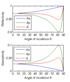
Figure 1: MATLAB plots of the reflectivities and absorptivities as a function of angle of incidence using fresnelplot (in this particular case for copper at a wavelength of 1.06mm).
Optical and dielectric constants
[e1,e2] = oc2dc (n,k)DESCRIPTION: converts the complex refractive index n+ik to the complex dielectric constant e1+ie2.
INPUT: n-refractive index, k-extinction coefficient
OUTPUT: e1-real part of the dielectric constant, e2-imaginary part of the dielectric constant
INPUT: n-refractive index, k-extinction coefficient
OUTPUT: e1-real part of the dielectric constant, e2-imaginary part of the dielectric constant
[n,k] = dc2oc (e1,e2)
DESCRIPTION: converts the complex dielectric constant e1+ie2 to the complex refractive index n+ik.
INPUT: e1-real part of the dielectric constant, e2-imaginary part of the dielectric constant
OUTPUT: n-refractive index, k-extinction coefficient
INPUT: e1-real part of the dielectric constant, e2-imaginary part of the dielectric constant
OUTPUT: n-refractive index, k-extinction coefficient
Surface normals and inclination angles
[nx,ny] = normals1D (f,x)DESCRIPTION: estimates local surface normals of a 1D surface profile y=f(x) using central differences of a 3-point neighbourhood with the reciprocal of the squared Euclidean distance as a weighting factor.
INPUT: f-surface heights, x-surface points
OUTPUT: nx-x components or surface normals, ny-y components or surface normals
INPUT: f-surface heights, x-surface points
OUTPUT: nx-x components or surface normals, ny-y components or surface normals
[nx,ny,nz] = normals2D (f,x,y)
DESCRIPTION: estimates local surface normals of a 2D surface z=f(x,y) using central differences of a 3-point neighbourhood with the reciprocal of the squared Euclidean distance as a weighting factor.
INPUT: f-surface heights, x-surface points, y-surface points
OUTPUT: nx-x components or surface normals, ny-y components or surface normals, nz-z components or surface normals
INPUT: f-surface heights, x-surface points, y-surface points
OUTPUT: nx-x components or surface normals, ny-y components or surface normals, nz-z components or surface normals
iaplot1D (f,x,plotopt) - (requires normals1D)
DESCRIPTION: plots the distribution of the inclination angles of a 1D rough surface profile z=f(x).
INPUT: f-surface heights, x-surface points, plotopt-plotting option (type 'plot' for plotting the continuous distribution or 'hist' for plotting a histogram of the discrete distribution)
OUTPUT: plot of the distribution of inclination angles
INPUT: f-surface heights, x-surface points, plotopt-plotting option (type 'plot' for plotting the continuous distribution or 'hist' for plotting a histogram of the discrete distribution)
OUTPUT: plot of the distribution of inclination angles
iaplot2D (f,x,y,plotopt) - (requires normals2D)
DESCRIPTION: plots the distribution of the inclination angles of a 2D rough surface z=f(x,y).
INPUT: f-surface heights, x-surface points, y-surface points, plotopt-plotting option (type 'plot' for plotting the continuous distribution or 'hist' for plotting a histogram of the discrete distribution)
OUTPUT: plot of the distribution of inclination angles
INPUT: f-surface heights, x-surface points, y-surface points, plotopt-plotting option (type 'plot' for plotting the continuous distribution or 'hist' for plotting a histogram of the discrete distribution)
OUTPUT: plot of the distribution of inclination angles
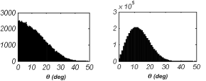
Figure 2: MATLAB plots of the inclination angle distributions for 1D surface profiles using iaplot1D (left) and for 2D surfaces using iaplot2D (right), both surfaces with the same rms height and correlation length illustrating the difference in 2D and 3D scattering.
References:
[1] Modest, M.: "Radiative Heat Transfer", Elsevier Science, 2nd Edition (2003).